PIVMat Frequently Asked Questions

PIVMat Frequently Asked Questions

If you have a question which is not answered here, or a suggestion on how you would improve this section, please feel free to send an e-mail to the author, moisy@fast.u-psud.fr.

Basic questions

How to import and display velocity fields?

Go to the directory where your files are stored (VEC, VC7, MAT files or others), and type
```
v = loadvec('B00001.VC7');
```
to load a single file (here 'B00001.VC7'). To load all the files in the current directory, type e.g.
```
v = loadvec('*.VC7');
```
To load only files 1 to 10, use
```
v = loadvec(1:10);
```
To display the fields, type
```
showf(v);
```
There are several shortcuts: For instance, this will display a movie of all the files in the current directory:
```
showf('*.VC7');
```
See the page Importing data into PIVMat to learn more.
How to have a quick help on a function from the PIVMat toolbox?

To get information about the function loadvec, type
```
doc loadvec
```
(open the help browser with the help for this function), or
```
help loadvec
```
(display the text of the help in the command window). If you don't know what you look for, have a look to the Function by category section from the PIVMat main page:
```
docpivmat
```
What Matlab knowledge should I have to use the PIVMat toolbox?

You should be familiar with the basic Matlab syntax, especially the use of colons (:) to index arrays, and the use of structures and structure arrays.
My velocity fields are noisy, how to smooth?

Use filterf or bwfilterf, eg:
```
showf(filterf(v,2));
```
How can I display the vorticity from a velocity field?

First load your vector field with
```
v = loadvec('B00001.VC7');
```
Then display it with the background option 'rot'
```
showf(v,'rot');
```
Another way to do this is to create a scalar field curl,
```
curl = vec2scal(v,'rot');
```
and then to display it:
```
showf(curl);
```
Before computing the vorticity field, you will probably want to filter your vector field:
```
showf(filterf(v,1),'rot');
```
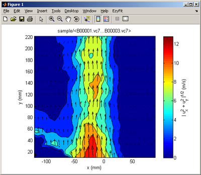
Many other vector-to-scalar conversions (divergence, kinetic energy, velocity derivatives...) are available from vec2scal.
I just want to display the first 10 fields of my set!

You may load all the vector fields and display only the ones you want:
```
v = loadvec('*.VC7');
```
Just refer to the fields you want with v(n), where n is a number (eg, showf(v(4)) displays the field #4).
If you want to refer to a range of fields, n may be an array, like [1 3 8], or 1:10 (type doc colon to learn more about Matlab's colon (:)). So, to display only the first 10 fields, type
```
showf(v(1:10));
```
If you want to skip one field every 2, type
```
showf(v(1:2:10));
```
You may also only load the fields you want, by using wildcards (*) and/or brackets []. In order to load only the files B00001.VC7 to B00010.VC7, type
```
v = loadvec('B[1:10].VC7');
```
See rdir for details about the usage of the brackets []. There is also a shortcut to do so,
```
v = loadvec(1:10);
```
(in this case, the 10 first files are loaded in the alphabetically-ordered set of files of the current directory).
See the page Importing data into PIVMat to learn more.
Can I import an IMX or IM7 image file?

Yes, loadvec accepts IMX/IM7 files; they will be considered as normal scalar fields, ie: use showf to display them. You may use colormap gray to use a black-and-white color map, which is usually more suitable for images.
Can I import a vector field saved in a TXT or DAT file?

Yes. Simply use loadvec (see also loadpivtxt). However, if you work with DaVis, it is better to import directly the VC7 files: it is faster, and these files contain many additional informations.
Why all the vectors are not displayed with showf?

A vector field is a bit confusing when too many vectors are present in a field. By default, showf displays at most 32 vectors in each direction, whatever the vector field resolution. This can be changed using the 'Spacing' option of showf, eg:
```
showf(v,'norm','spacing',2);
```
You may also display specify different spacing in the x- and y-direction:
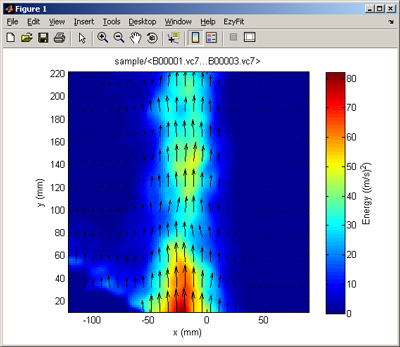
```
showf(filterf(v,1.5),'ken','spacing',[4 12]);
```
What is the difference between the ReadIMX package provided by LaVision and the PIVMat toolbox?

The ReadIMX package provided by LaVision allows to import a (single) VC7/IMX/IM7 file from Davis into Matlab, and to display it. That's all.
The PIVMat toolbox is based on the function readimx from the ReadIMX package, but offers much more. Note that the ReadIMX package has to be installed separately for the PIVMat toolbox to work correctly (see the Installation page).
Can I import 3D velocity fields (Stereoscopic PIV)?

PIVMat is compatible with stereo (3-components) velocity fields only for DaVis files.

Advanced questions

How to plot lines of iso-velocity?

Use showf with the option 'contour' or 'contourf', e.g.
```
showf(v,'contourf',8,'spacing',[4 12]);
```
How to navigate into a set of fields?

First load your vector fields with
```
v = loadvec('*.VC7');
```
Display a movie of your fields,
```
showf(v);
```
You can enter into the 'pause' mode by pressing the space bar. Then navigate using the left or right arrow. Press the space bar to run the movie again. Press ESC to escape. Use option 'loop' to run the movie in a loop. You may also directly enter into the 'pause' mode by specifying the option 'pause'. See showf.
How are stored the vector fields in Matlab?

A vector field loaded with
```
v = loadvec('B00001.VC7');
```
is stored into a "PIVMat structure" v. A PIVMat structure is a variable that contains several variables of different types (see 'Data Types > Structures' in the Matlab help). The structure v contains the axis, the velocity components, the field names etc. If the fields originate from DaVis, the PIVMat structure also contains several attributes saved by DaVis (acquisition time, etc). For instance, the x-component of the velocity field is stored in the matrix vx of the structure v. In order to refer (eg, plot, display, modify...) to the x-component of the velocity at the point (i,j), you should type
```
v.vx(i,j)
```
If you have loaded several fields in a single structure v, e.g. with
```
v = loadvec('*.VC7');
```
then v is now a "structure array". You can refer to the (i,j) point of the x-component of the n-th vector field with
```
v(n).vx(i,j)
```
See Data Organization in PIVMat for a full description of PIVMat structures.
How can I plot a velocity profile from a vector field?

The velocity components are stored in the two arrays vx and vy of the structure v loaded by loadvec (see question above). So, to plot a velocity profile along the horizontal line at height y=12 (in mesh units), type
```
plot(v.x, v.vx(:,12))
```
(type doc colon to learn more about Matlab's colon (:)).
You may also plot the velocity profile averaged over several horizontal lines, for instance between y=12 and y=14 (in mesh units):
```
plot(v.x, mean(v.vx(:,10:14),2))
```
How can I plot a vorticity profile?

First compute the vorticity from a velocity field,
```
vort = vec2scal(v, 'rot');
```
Then follow the same procedure as above. The vorticity is contained into the variable w of the structure vort:
```
plot(vort.x, vort.w(:,12))
```
How can I create a MP4 / AVI movie file from my vector fields?

(New Pivmat 4.10) You can use showf to create MP4 / AVI movies.
First load your fields, e.g.
```
v = loadvec('*.VC7');
```
Create a VideoWriter object:
```
vid = VideoWriter('mymovie.mp4');
```
Call showf and close the movie
```
showf(v, 'savevideo', vid, 'rot', 'clim', [-3 3]);
close(vid);
```
Using a very large number of files may produce 'out of memory'. An alternative method consists in loading the files one by one, without storing them in a PIVMat structure:
```
vid = VideoWriter('mymovie.avi');
imvectomovie('*.IM7', vid, 'clim', 2000);
close(vid);
```
What is the mean kinetic energy of my field?

First compute the kinetic energy of your field v
```
ke = vec2scal(v, 'ken');
```
Then call the function statf
```
st = statf(ke);
```
What you want is the mean of ke:
```
st.mean
```
How to save fields processed with Matlab?

Suppose you have computed complex operations from a series of vector fields,
```
v=loadvec('*.vc7');
v=shiftf(extractf(v,[10 10 100 100],'phys'),'center');
fv=bwfilterf(v, 2, 8);
curl=vec2scal(fv, 'rot');
```
Then you can save your final set of scalar fields curl in a Matlab file,
```
save('mycurl.mat','curl');
```
You can retrieve your fields using
```
rot = loadvec('mycurl.mat');
```
Note that you can also load your fields using the standard Matlab's load function,
```
load mycurl
```
In this case, the field name (here 'curl') will be the same as the one specified to the save command.
Where is stored the acquisition time of a vector field?

The acquisition time, and other parameters of Davis, are stored in the variable Attribute of a field v. Use the function getattribute to get the value of a given attribute. For instance, for VC7 files (from Davis 7), the time acquisition is stored in the attribute AcqTimeSeries0:
```
t = getattribute(v,'AcqTimeSeries0');
```
returns the time t of v (or the array of times, if v is an array of fields). You may also use the function getpivtime, which is a shortcut for this attribute.
How can I compute the rms (root-mean-square) of a series of vector fields?

First load your vector fields with
```
v = loadvec('*.vc7');
```
Then use averf with the following output arguments and plot the result:
```
[af rms] = averf(v);
showf(rms);
```
How can I plot the velocity at some given point as a function of time?

First load your vector fields with
```
v = loadvec('*.vc7');
```
Then store the x and y components of the velocity at a given point, say (X,Y) = (20, 40) mm, using probef:
```
[ux,uy] = probef(v, 20, 40);
```
then plot the result
```
plot(1:length(ux), ux)
```
If you use DaVis files, you can use getpivtime and getattribute to get the time stored in each file.
How can I plot a spatio-temporal diagram from a vector field?

You should build a matrix, say d(i,j), where the quantity of interest is a vector (index i) and the time is along j. Once the vector fields v and the time t are obtained (see the above question), type
```
for j=1:length(v)
   d(:,j) = v(j).vx(:,12);
end;
imagesc(v(1).x, t, d');
xlabel('x'); ylabel('t');
```
What are all the successive operations performed on a given field?

Among the variables stored in the structure v, one is called "history". This variable is a cell array of strings, and each operation adds a new string to this cell array, which describes this operation. For instance, suppose you do
```
v=loadvec('B00001.vc7');
v=shiftf(extractf(v,[10 10 100 100],'phys'),'center');
fv=bwfilterf(v, 2, 8);
curl=vec2scal(fv, 'rot');
```
If you type
```
curl.history
```
you obtain the following cell array of strings:
```
    'loadvec('B00001.vc7')'
    'extractf(ans, [10 10 100 100], 'phys')'
    'shiftf(ans, 'center')'
    'bwfilterf(ans, 2, 8, 'low')'
    'vec2scal(ans, 'rot', 'nonzero')'
```
In this list, ans refers to the result of the previous operation. See Programming > Data Types > Cell arrays in the Matlab help to learn more about cell arrays.
Should I always use loadvec to display/process my set of files?

Most of the time you have to first load your files, e.g. v=loadvec('*.vc7'), and then you perform your computations from v, e.g. showf(filterf(v,2)). However, a number of operations can be performed directly from the files themselves. For example, try
```
filterf('*.vc7',2);
```
When a string is passed as the first argument of filterf, the file is first loaded by loadvec. When no output argument is specified, then showf is automatically called. Numeric arguments may also be used:
```
averf(1:10);
```
displays the average of the 10 first files on the current directory.
Can I display the current time in my movie?

Yes, you may use the option 'title' in showf , e.g.
```
showf(v,'loop','title','%s, t = %t s');
```
In this example, the string '%s' is replaced by the setname (i.e. the directory name where were stored the files), and the string '%t' is replaced by the current time of each field, as obtained by getpivtime.

Expert questions...

I have to process 1000 vector fields but I haven't enough memory!

Loading a large amount of fields into a single big structure with v=loadvec('*.vc7') is not always possible due to lack of memory, so you should process your files one by one without storing the whole set.
For simple operations, you may use the function batchf for this purpose
```
batchf('*.vc7','showf','norm');
```
This calls sequentially the function showf for each file matching '*.vc7' in the current directory, passing the additional parameter 'norm'.
More complex operations should be performed using a for loop. This example plots the kinetic energy versus file number of all the VC7 files in the current directory:
```
file = rdir('*.vc7');
for i=1:length(file)
   v = loadvec(file{i});
   st = statf(vec2scal(v,'ken'));
   k(i) = st.mean;
end;
plot(k);
```
(note the use of curly braces {} for cell arrays of strings - see rdir for details).
I want to load n sets of p vector fields!

If you want to concatenate n sets of p vector fields into a single big structure v of size n*p, assuming the fields are stored into directories named myset1, myset2..., use
```
v = loadvec('myset*/*.vc7');
```
However, you loose the ordering of the files doing so. If now you prefer to store your fields into a 2D array of fields, use loadarrayvec
```
v = loadarrayvec('myset*','*.vc7');
```
Use something like showf(v(1,:)) to display all the fields from the first directory, or showf(v(:,1)) for all the first fields from each directory.
How to compute ensemble averages from my n sets of p fields?

First load your fields with (see previous question):
```
v = loadarrayvec('myset*','*.vc7');
```
Then you can average all the first fields from each directory, all the second fields from each directory, etc:
```
for i=1:size(v,1),
    af(i) = averf(v(i,:));
end;
showf(af);
```
How to compute scalar fields other than the default ones proposed in vec2scal?

vec2scal allows to convert vector fields into most classical scalar fields of interest (vorticity, divergence etc.) For more exotic operations, you may use operf. You may also write your own .m file, starting from a basic scalar field. For instance, suppose you want to compute a scalar field given by 2*vx + vy^2:
```
function res = strangefield(v)
res = vec2scal(v,'norm');
res.w = 2*v.vx + v.vy.^2;
res.namew = 'strange field';
```
Then simply call your function with:
```
showf(strangefield(loadvec('B00001.VC7')));
```
How to load multiframe fields?

Davis' multiframe fields are not supported by PIVMat. loadvec will load only the first frame of a field. You should first use Davis to expand your multiframe buffer into several single-frame buffers, and then load the resulting buffers as usual with loadvec.
What is the variable ysign?

The calibration of the Y-axis may be upward or downward. In Matlab, the natural way to plot a matrix using the function image is using a downward Y-axis (defaut mode axis ij, for matrix representation). When using upward an Y-axis (mode axis xy, for function representation), Matlab re-orders the Y vector, so the Y-axis is wrong.
The variable ysign in the structure v is a string, that may be 'Y axis downward' or 'Y axis upward', which is determined by loadvec when loading the field.
See also the page Data Organization in PIVMat to learn more about the matrix indexing convention in PIVMat.

2005-2018 PIVMat Toolbox