The "dispersion relation" toolbox for surface waves

F. Moisy, 28 april 2010.

Laboratory FAST, University Paris Sud.

Contents

About the dispersion relation of surface waves

This toolbox simply provides an easy way to work with the dispersion relation of surface waves, given by

   omega(k) = sqrt ( tanh(k*h0) * (g*k + gamma*k^3/rho))

where omega is the pulsation (in rad/s), k the wavenumber (in 1/m), h0 the depth (in m), g the gravity (in m^2/s), gamma the surface tension (in N/m) and rho the fluid density (in kg/m^3).

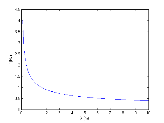
The following example simply plots the wave frequency as a function of wavelength:

lambda = 0:0.1:10;  % wavelength (in m)
freq = omega(2*pi./lambda)/(2*pi);
plot(lambda,freq);
xlabel('\lambda (m)');
ylabel('f (Hz)');

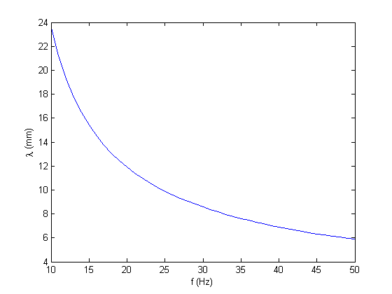
Inverting the dispersion relation

The function kfromw allows one to invert the dispersion relation, i.e. to give the value of omega for a given value of k.

For infinite depth, kfromw inverts the cubic polynomial. For finite depth, a zero-finding method is used, starting from the infinite depth solution.

freq = 10:50;  % in Hz;
lambda = 2*pi./kfromw(2*pi*freq);
plot(freq, 1000*lambda);
xlabel('f (Hz)');
ylabel('\lambda (mm)');

Setting the wave parameters

By default, the physical parameters (liquid densities, surface tension, etc.) are set for an air-water interface under usual conditions, with a water layer of infinite depth ("deep water waves"). The default settings are given by the function wave_parameter:

p = wave_parameter

p = 

        g: 9.8100
    gamma: 0.0720
      rho: 1000
       h0: Inf

The structure p can be passed as an input argument to omega and kfromw.

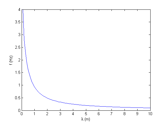
The default settings can be changed as follows: here the surface tension is set to 0.06 N/m and the depth to 0.1 m:

p = wave_parameter('gamma',0.05,'h0',0.1)

p = 

        g: 9.8100
    gamma: 0.0500
      rho: 1000
       h0: 0.1000

Re-do the same plot as above with the new settings:

lambda = 0:0.1:10;
freq = omega(2*pi./lambda, p)/(2*pi);     % note the second parameter p
plot(lambda,freq);
xlabel('\lambda (m)');
ylabel('f (Hz)');

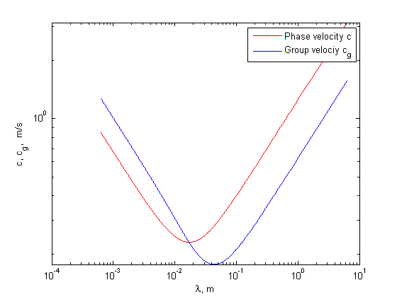
Phase and group velocity

The function omega also returns, as additional output arguments, the phase and group velocity of the wave:

k = linspace(1,1e4,1e4);
[w,c,cg] = omega(k);
lambda = 2*pi./k;
loglog(lambda,c,'r-',lambda,cg,'b-');
xlabel('\lambda, m')
ylabel('c, c_g,  m/s');
legend('Phase velocity c','Group velociy c_g');

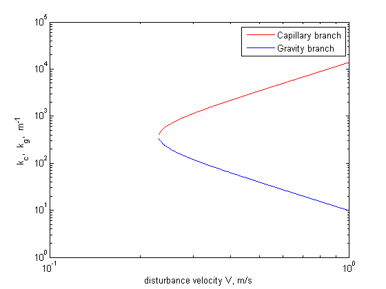
Kelvin wake

A last function of the toolbox, kckg, returns the capillary wavenumber kc and gravity wavenumber kg for a given phase velocity U. This is useful in the problem of the Kelvin wake, in which the range of excited wavenumbers is given by equating the disturbance velocity and the phase velocity. Here again, the wave parameters stored in the structure p may be passed as an additional input argument to kckg.

v = linspace(0,1,1000);  % disturbance velocity, m/s
[kc, kg] = kckg(v);      % wavenumbers selected by the velocity
loglog(v,kc,'r-',v,kg,'b-');
xlabel('disturbance velocity V, m/s');
ylabel('k_c,  k_g,  m^{-1}')
xlim([.1 1])
legend('Capillary branch','Gravity branch');

Rayleigh-Taylor instability

If the gravity is negative, omega may return a complex value. The imaginary part corresponds to the growthrate of the Rayleigh-Taylor instability (a denser fluid above a lighter fluid).

p = wave_parameter('g',-10);
k = linspace(100, 1000, 100);
s = omega(k,p);
lambda = 2*pi./k;
plot(1000*lambda,imag(s),'b',1000*lambda,real(s),'r')
xlabel('\lambda (mm)');
ylabel('1/s');
legend('Growth rate (unstable)','Pulsation \omega (stable)');

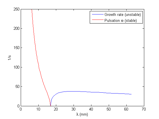
Here the most unstable wavelength is k = 29 mm.

More?

To learn more about this toolbox, see the help:

help dispersion_relation

  Dispersion Relation Toolbox (F. Moisy)
  Version 1.01 28-Apr-2010
 
  Dispersion relation
    omega          - Dispersion relation w(k) for surface waves
    kfromw         - Inverse dispersion relation k(w) for surface waves
    wave_parameter - Set the parameters for the dispersion relation
    kckg           - Wavenumbers selected by a given velocity
 
  Various plot examples
    plot_lambda    - Wavelength versus frequency
    plot_c         - Phase and group velocities versus wavenumber.
    plot_kckg      - Gravity and capillary wavenumbers of the Kelvin wake

Published with MATLAB® 7.10