Computing a fractal dimension with Matlab: 1D, 2D and 3D Box-counting
F. Moisy, 9 july 2008.
Laboratory FAST, University Paris Sud.
Contents
About Fractals and box-counting
A set (e.g. an image) is called "fractal" if it displays self-similarity: it can be split into parts, each of which is (at least approximately) a reduced-size copy of the whole.
A possible characterisation of a fractal set is provided by the "box-counting" method: The number N of boxes of size R needed to cover a fractal set follows a power-law, N = N0 * R^(-DF), with DF<=D (D is the dimension of the space, usually D=1, 2, 3).
DF is known as the Minkowski-Bouligand dimension, or Kolmogorov capacity, or Kolmogorov dimension, or simply box-counting dimension.
To learn more about box-counting, fractals and fractal dimensions:
- http://en.wikipedia.org/wiki/Fractal
- http://en.wikipedia.org/wiki/Box_counting_dimension
- http://mathworld.wolfram.com/Fractal.html
- http://mathworld.wolfram.com/CapacityDimension.html
About the 'boxcount' package for Matlab
The following examples illustrate how to use the Matlab package 'boxcount' to compute the fractal dimension of 1D, 2D or 3D sets, using the 'box-counting' method.
The directory contains the main function 'boxcount', three sample images, and an additional function 'randcantor' to generate 1D, 2D and 3D generalized random Cantor sets.
Type 'help boxcount' or 'help randcantor' for more details.
Box-counting of a 2D image
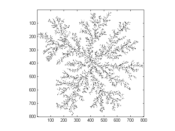
Let's start with the image 'dla.gif', a 800x800 logical array (i.e., it contains only 0 and 1). It originates from a numerical simulation of a "Diffusion Limited Aggregation" process, in which particles move randomly until they hit a central seed. (see P. Bourke, http://local.wasp.uwa.edu.au/~pbourke/fractals/dla/ )
c = imread('dla.gif');
imagesc(~c)
colormap gray
axis square
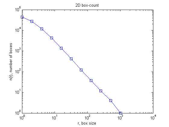
Calling boxcount without output arguments simply displays N (the number of boxes needed to cover the set) as a function of R (the size of the boxes). If the set is a fractal, then a power-law N = N0 * R^(-DF) should appear, with DF the fractal dimension (Kolmogorov capacity).
boxcount(c)
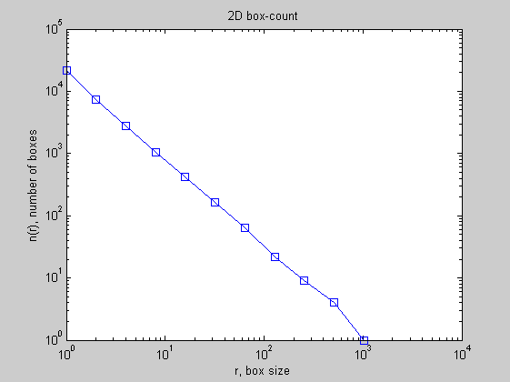
The result of the box count can be obtained using:
[n, r] = boxcount(c)
loglog(r, n,'bo-', r, (r/r(end)).^(-2), 'r--')
xlabel('r')
ylabel('n(r)')
legend('actual box-count','space-filling box-count');
n =

  Columns 1 through 7

       44000       27466       11786        4265        1386         421         121

  Columns 8 through 11

          37          12           4           1


r =

  Columns 1 through 7

           1           2           4           8          16          32          64

  Columns 8 through 11

         128         256         512        1024
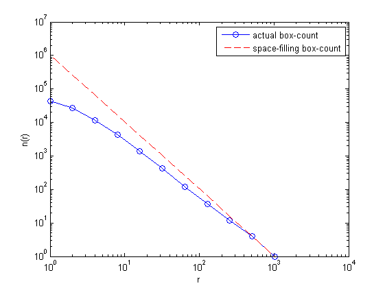
The red dotted line shows the scaling N® = R^-2 for comparision, expected for a space-filling 2D image. The discrepancy between the two curves indicates a possible fractal behaviour.
Local scaling exponent
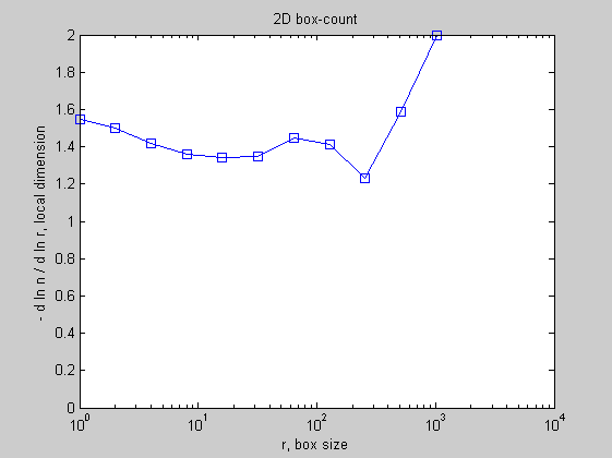
If the set has some fractal properties over a limited range of box size R, this may be appreciated by plotting the local exponent, D = - d ln N / ln R. For this, use the option 'slope':
boxcount(c, 'slope')
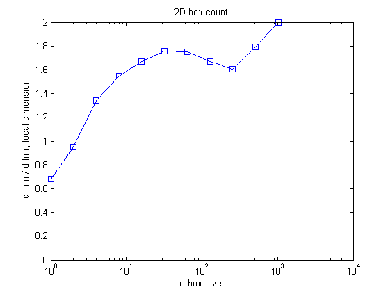
Strictly speaking, the local exponent is not constant, but lies in the range [1.6 1.8].
Let's try now with another image, the so-called Apollonian gasket (Wikipedia, http://en.wikipedia.org/wiki/Image:Apollonian_gasket.gif ). The background level is 198 for this image, so this value is used to binarize the image:
c = imread('Apollonian_gasket.gif');
c = (c<198);
imagesc(~c)
colormap gray
axis square
figure
boxcount(c)
figure
boxcount(c,'slope')
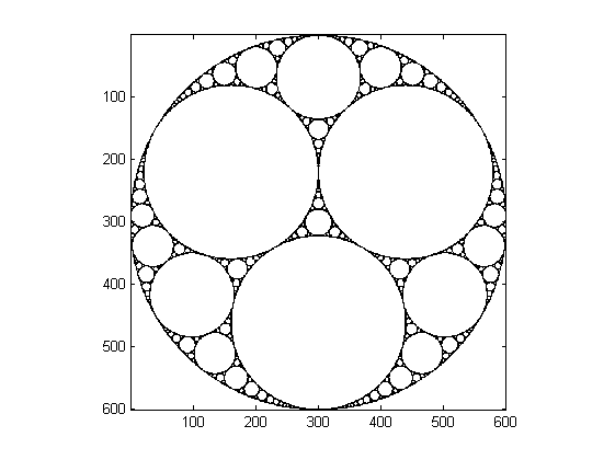
The local slope shows that the image is indeed approximately fractal, with a fractal dimension DF = 1.4 +/- 0.1 for scales R < 100.
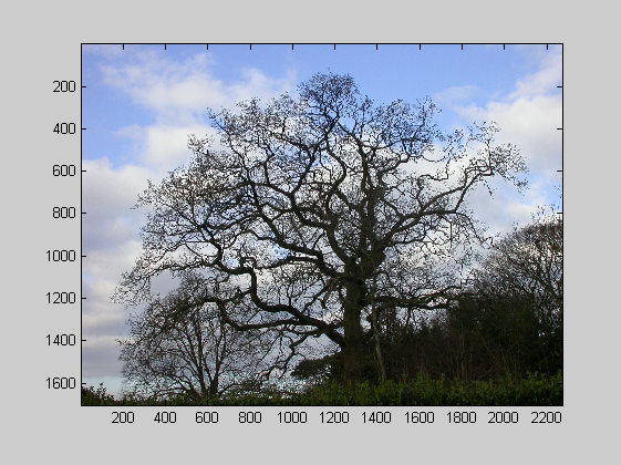
Box-counting of a natural image.
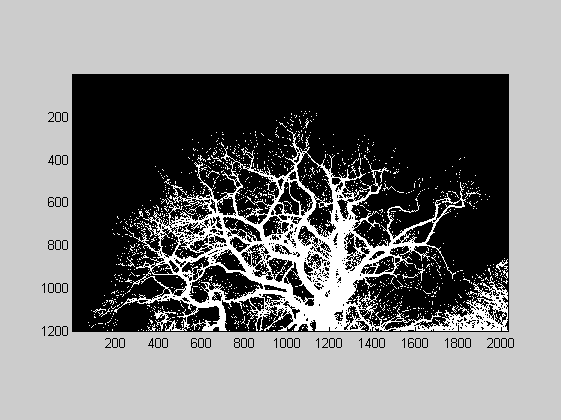
Consider now this RGB (2272x1704) picture of a tree (J.A. Adam, http://epod.usra.edu/archive/images/fractal_tree.jpg ):
c = imread('fractal_tree.jpg');
image(c)
axis image
Let's extract a rectangle in the blue (3rd) plane, and binarize the image for levels < 80 (white pixels are logical 'true'):
i = c(1:1200, 120:2150, 3);
bi = (i<80);
imagesc(bi)
colormap gray
axis image
[n,r] = boxcount(bi,'slope');
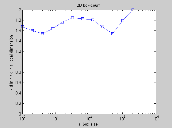
The boxcount shows that the local exponent is approximately constant for less than one decade, in the range 8 < R < 128 (the 'exact' value of Df depends on the threshold, 80 gray levels here):
df = -diff(log(n))./diff(log(r));
disp(['Fractal dimension, Df = ' num2str(mean(df(4:8))) ' +/- ' num2str(std(df(4:8)))]);
Fractal dimension, Df = 1.801 +/- 0.06394
Generalized random Cantor sets
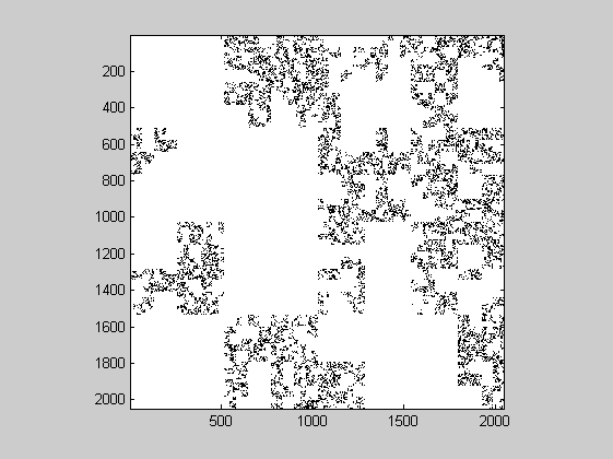
Fractal sets may be obtained from an IFS (iterated function system). For example, the function 'randcantor' provided with the package generates a 1D, 2D or 3D generalized random Cantor set. This set is obtained by iteratively dividing an initial set filled with 1 into 2^D subsets, and setting each subset to 0 with probability P. The result is a fractal set (or "fractal dust") of dimension DF = D + log(P)/log(2) < D.
The following example generates a 2048x2048 image with probability P=0.8, i.e. fractal dimension DF = 1.678.
c = randcantor(0.8, 2048, 2);
imagesc(~c)
colormap gray
axis image
Let's see its box-count and local exponent
boxcount(c)
figure
boxcount(c, 'slope')
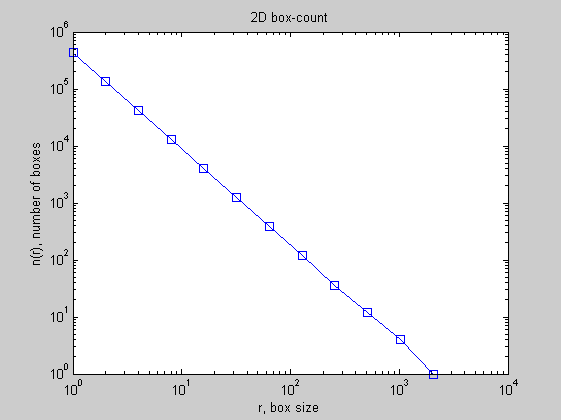
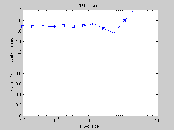
For such set generated by an iterated scheme, the local slope shows as expected a well defined plateau, around DF = 1.7.
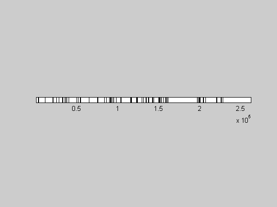
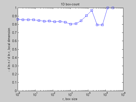
1D random Cantor set
1D random Cantor sets may also be generated. Here, a 2^18 = 262144 long set with P = 0.9 and expected fractal dimension DF = 1 + log(P)/log(2) = 0.848:
tic
c = randcantor(0.9, 2^18, 1, 'show');
figure
boxcount(c, 'slope');
toc
Elapsed time is 4.022846 seconds.
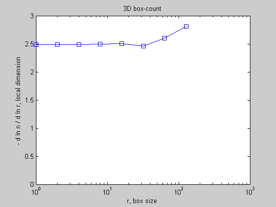
3D random Cantor set
Now a 3D random Cantor set of size (2^7)^3 = 128^3 with P = 0.7 and expected fractal dimension DF = 3 + log(P)/log(2) = 2.485. Note that 3D sets cannot be displayed using randcantor.
tic
c = randcantor(0.7, 2^7, 3);
toc
tic
boxcount(c, 'slope');
toc
Elapsed time is 12.197119 seconds.
Elapsed time is 0.186419 seconds.
More?
That's all. To learn more about this package, type:
help boxcount.m
 BOXCOUNT  Box-Counting of a D-dimensional array (with D=1,2,3).
    [N, R] = BOXCOUNT(C), where C is a D-dimensional array (with D=1,2,3),
    counts the number N of D-dimensional boxes of size R needed to cover
    the nonzero elements of C. The box sizes are powers of two, i.e.,
    R = 1, 2, 4 ... 2^P, where P is the smallest integer such that
    MAX(SIZE(C)) <= 2^P. If the sizes of C over each dimension are smaller
    than 2^P, C is padded with zeros to size 2^P over each dimension (e.g.,
    a 320-by-200 image is padded to 512-by-512). The output vectors N and R
    are of size P+1. For a RGB color image (m-by-n-by-3 array), a summation
    over the 3 RGB planes is done first.

    The Box-counting method is useful to determine fractal properties of a
    1D segment, a 2D image or a 3D array. If C is a fractal set, with
    fractal dimension DF < D, then N scales as R^(-DF). DF is known as the
    Minkowski-Bouligand dimension, or Kolmogorov capacity, or Kolmogorov
    dimension, or simply box-counting dimension.

    BOXCOUNT(C,'plot') also shows the log-log plot of N as a function of R
    (if no output argument, this option is selected by default).

    BOXCOUNT(C,'slope') also shows the semi-log plot of the local slope
    DF = - dlnN/dlnR as a function of R. If DF is contant in a certain
    range of R, then DF is the fractal dimension of the set C. The
    derivative is computed as a 2nd order finite difference (see GRADIENT).

    The execution time depends on the sizes of C. It is fastest for powers
    of two over each dimension.

    Examples:

       % Plots the box-count of a vector containing randomly-distributed
       % 0 and 1. This set is not fractal: one has N = R^-2 at large R,
       % and N = cste at small R.
       c = (rand(1,2048)<0.2);
       boxcount(c);

       % Plots the box-count and the fractal dimension of a 2D fractal set
       % of size 512^2 (obtained by RANDCANTOR), with fractal dimension
       % DF = 2 + log(P) / log(2) = 1.68 (with P=0.8).
       c = randcantor(0.8, 512, 2);
       boxcount(c);
       figure, boxcount(c, 'slope');

    F. Moisy
    Revision: 2.10,  Date: 2008/07/09